This chapter describes the mathematics that CUBE Analyst uses. Topics include:

• Mathematical notation
• Introduction to the mathematics in CUBE Analyst
• Mathematical summary
• Extensions to the calculations

Mathematical notation

This section discusses mathematical notation. Topics include:

• Explaining the letters and symbols
• Notation used in the estimation equation

Explaining the letters and symbols

This section uses mathematical notation, which can look daunting for those who are not accustomed to it. So, first, a word of background explanation. The notation can be made to appear worse because of the use of greek letters and some specialist mathematical symbols. The problem is that the normal 26-letter Roman alphabet is not sufficient, even considering upper and lower case letters, and remembering that some letters have traditional mathematical meanings and associations. The mathematics which is presented here is only an extract of the full CUBE Analyst mathematics, which uses an even wider range of letters. Also, some of the traditional mathematical notations are cumbersome when used with vectors and matrices and their elements, as CUBE Analyst requires, hence it is better to use alternative forms.

This is mainly a pronunciation guide, but some of the symbols and letters are explained further:

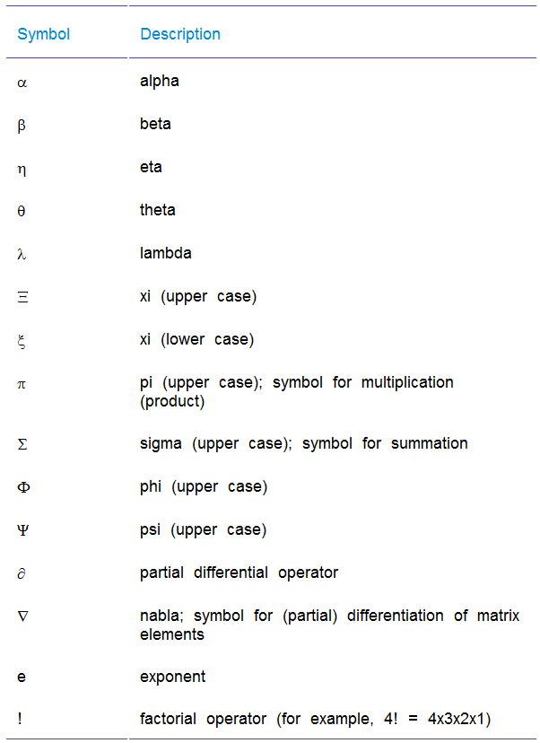
The notation P(x|X) implies the probability of x, given the value X. Similarly, L(x|X) is the likelihood of x, given X; M(x|X) refers to the log-likelihood of x, given X. Note the use of bold in the last example implies that x and X are multi-valued vectors (or matrices).

Notation used in the estimation equation

This notation is used in Introduction to the mathematics in CUBE Analyst and Mathematical summary.

Introduction to the mathematics in CUBE Analyst

The design of CUBE Analyst means that a user can estimate matrices simply by supplying the program with the appropriate input data and accepting the resulting matrix. However, it is valuable to have some understanding of how CUBE Analyst calculates the value of the estimated matrix cells; this insight both helps in providing confidence in the results and in guiding the approach to input data, such as setting confidence levels and considering the potential effects of extra data or improved data quality.

This section provides additional information about how CUBE Analyst computes matrix cells. Topics include:

• Main mathematical features
• Estimation equation
• Model parameters
• Maximum likelihood objective function
• Describing the variation in data
• Optimizer: Finding the minimum value

Main mathematical features

This section is intended to cater to those CUBE Analyst users who are interested in the detailed mathematical and statistical underpinnings of the estimation process. Users who are more interested in other aspects of the model should proceed to Chapter 5, “Data Preparation and Analysis.”

The basis of CUBE Analyst’s calculations is an application of the standard statistical approach known as the maximum likelihood method. This method allows estimates of a set of inputs to guide the estimates of a corresponding set of outputs; the estimates of the set of inputs are obtained from likelihood functions, which are expressions of probability distribution functions (pdfs) associated with the user’s input data. The outputs are calculated from an estimation equation, which must be provided. These points are further explained below.

Given the range of possible input data, the full mathematical expression of CUBE Analyst is complex, but it involves some principal components which we use to describe the essential features of CUBE Analyst. Mathematical summary explains the standard CUBE Analyst calculations by summarizing the main mathematical steps. Extensions to the calculations shows how additional features are accommodated in the calculations. This section continues with explaining CUBE Analyst’s mathematics in largely descriptive terms, while introducing the main equations. Throughout this section, the mathematical notation is defined Mathematical notation, where it is not otherwise clear from the text.

Estimation equation

The heart of the estimation is an equation (”estimation model”) whose output, T_ij, corresponds to the values of the cells of CUBE Analyst’s output matrix for trips between zones iand j. The form of this mathematical estimation model in CUBE Analyst is:

(1)

This equation contains the following elements:

•its output T_ij,

•some data items:

t_ij-Prior observation of trips between imageiand j

R_ijkProbability of trips between zones imageiand jusing screenline sitek(it is possible for a ”screenline” to correspond to a single count site, in suitable circumstances)

•some Model Parameters

ai, bj, XK.

- Implies the product of X_Kover all the screenline count sites K

If there is not_ij prior observation for movements between some or all possible origin-destination zone pairs, ij, then t_ijmay be calculated by CUBE Analyst from:

(2)

Equation (2) introduces further elements:

•One data item:

c_ij- the generalized cost of travel between zonesiand j

•Two model parameters:

,

It may be noted that screenlines are usually organized so that R_ijk=1 or 0. Also, because t_ijprovides an estimator of the output, as well as possibly being an input data item, it may also be considered as a model parameter. Hence, the t_ij data item is also referred to as N_ij. (That is, t_ij and N_ij are numerically identical, but are logically distinct.)

The form of equation (1) has been chosen primarily for reasons of convenience, and for the appropriateness of its form according to the data used in the estimation (as we discuss below). It is designed to be efficient is assisting information to be processed, but is not behavioral in nature. This implies that CUBE Analyst is suitable for estimating present day matrices, but not for forecasting which would require some behavioral assumptions.

Equation (2) is borrowed from the well-known gravity model that makes the behavioral assumption that people prefer lower cost journeys to higher cost ones, but are influenced by the level of trips generated by and attracted to different zones. This is a broad assumption; it means that cost data may be used where no other source of prior matrix data is available, but it is not a precise approach to estimating individual matrix cells.

Model parameters

For CUBE Analyst, therefore, the estimated matrix is entirely dependent on the values given to the model parameters. CUBE Analyst is thus, in effect, solely concerned to establish the most appropriate values for these model parameters. (CUBE Analyst’s calculations are in ”parameter space,” which accounts for some of the behavior that may be observed in CUBE Analyst’s output to the screen and log file while it is computing, where the values of the matrix may change in an apparently erratic manner.) CUBE Analyst’s calculations are mainly in the nature of a search for the ”best” model parameter values. Apart from the estimation equation itself, the main features of the CUBE Analyst calculations are:

•Directing the search for Model Parameters values — ”optimization”

•Deciding whether the new Model Parameter values are the ”best” — ”function evaluation”

We now describe the general issues for CUBE Analyst when setting model parameter values.

Unless the user supplies an input model parameter file (created either by an earlier run of CUBE Analyst), the model parameters are automatically initialized to 1.0. From equation (1), it may be seen that the initial estimate is identical to the prior matrix (or based on the cost matrix, equation (2), if no prior matrix value exists).

It is possible to compare the estimated matrix with all of the items of the user’s input data. For example, the sum of rows and columns of the estimated matrix may be compared with input trip ends (Mathematical summary shows this in mathematical terms for all data items). If the result of this comparison indicates that the current estimate is too low, then an improved estimated matrix may be achieved by increasing the value of, at least, some model parameters.

The ”problem” for CUBE Analyst is that there are many items of user data, implying many comparisons of the type just described; some of these comparisons may require the current estimate to be improved in one way (increased, say), while other comparisons need the estimate to be altered another way (decreased, say). The large number of model parameters provides the basis for reconciling these apparent conflicts;by definition there are (2 x the number of zones) model parameters provided by the a_is and the b_js alone. It may be demonstrated that these are sufficient for equation (1) to define any possible combination of positive, non-zero matrix cell values. Hence, if, by some means, suitable values of the model parameters may be found, equation (1) can produce a matrix which is consistent with all of the user’s input data. That is, at least, if the input data is self-consistent in the first place.

Of course, this consistency is never the case in real applications of CUBE Analyst, and the best that may be hoped for is to estimate the matrix which is most likely, given the user’s input data. Achieving this ”most likely” result is the next main topic to discuss, but we will stay with model parameters to make a few more points.

In principle, there is nothing particular to distinguish the set of model parameters; mathematically, they are equal and each may be affected by any item of data. However, the form of the estimation equation allows parameters to be associated naturally with different types of data such as:

a_i,b_j- Trip ends, for trips generated at zone i and attracted to zone j

X_K- Counts on screenline site K

,- Trip c information

- Prior trip matrix

This association is useful to the optimizer in reflecting the different (quality) characteristics of the data sets. The nominally redundant X_K parameters provide extra ”degrees of freedom” to handle data inconsistencies. This is useful, as the matrix cells affected by a set of screenline data are precisely defined by the R_ijK routing information.

Maximum likelihood objective function

When CUBE Analyst establishes values for the model parameters, it requires a criterion to determine if the corresponding Tij estimates either are ”correct” or are ”better” than another set of model parameter values. This criterion is provided by a mathematical equation called an objective function. The objective function, M, for CUBE Analyst has the following form:

(3)

where:

h- is an estimated data item

H- is an observed data item

- is the confidence level associated with H

Notation used in the estimation equation shows which itemsH and hcan represent but, in general terms,H is the input data which the user supplies and h is the corresponding value implied by the estimated matrix.

We have already discussed how the form of the estimation equation (1) has been determined for reasons of effectiveness, but which remain essentially arbitrary; also, how equation (2) derives a weak behavioral basis from the gravity model. It is therefore important to appreciate that in contrast, the objective function, equation (3), is the result of a statistically rigorous procedure, namely the maximum likelihood method.

The consequence of this is a guarantee, subject to some qualifications which we consider below, that the estimated matrix is the statistically most likely, given the data supplied by the user. The ”correctness” of the estimate remains, of course, dependent on the quality of the input data. Maximum likelihood theory shows that the most likely values are indicated when M in equation (3), which is negative, reaches its minimum possible value. (For reasons of computational convenience, CUBE Analyst minimizes the negative of the ”log-likelihood” objective function, rather than maximizing the positive version, as the name ”maximum likelihood” might suggest.)

The qualifications mentioned before respectively concern the input data sets representing ”independent observations,” which is not normally a problem for CUBE Analyst users, and of the input data being described by a probability distribution function, which we now discuss. The derivation of equation (3) for the objective function is outlined in Mathematical summary.

Describing the variation in data

The maximum likelihood method assumes that each item of input data represents an observation from a random distribution of possible values, but where the variation of values may be described by a probability distribution function. That is when the user supplies CUBE Analyst with, say, a screenline traffic count value of 1684 vph; this is not considered to be the count for that screenline but, rather, a sample from a distribution. It is common experience that counting the same screenline on another, but equivalent occasion (for example, the same time the following week) will provide another count value, say 1739 vph, simply on account of the random variation which is inherent in all traffic (and passenger) data.

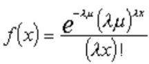
The assumption is made, therefore, that all input data for CUBE Analyst is subject to variation which may be described by the Poisson probability distribution function (pdf).

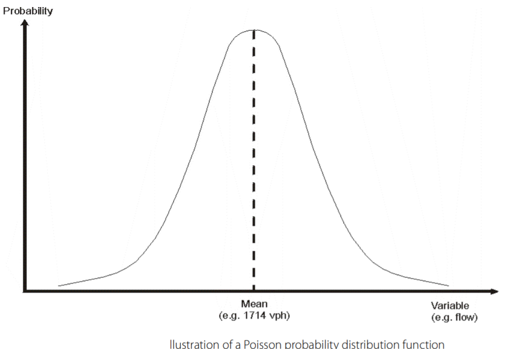
The Poisson is a well-known pdf, often associated with data which can involve many ”events” (for example, 1684 vehicles passing an observer in an hour). It has the statistical property that its mean equals its variance. This is valuable for data such as count information where the variation of 100 vph is significant when the mean figure is 200 vph, but not when it is 1000 vph; alternatively, a 10% variation implies many vehicles on a mean of 5000 vph, but not on 50 vph. The Poisson distribution reflects these changes in significance in an appropriate way.

During the original development of CUBE Analyst, alternative assumptions about the pdf used to describe data variation were reviewed; the Log-Normal distribution for example, but these were considered only to add complexity, rather than accuracy. It is usually that case that the Poisson is a good way of describing traffic and passenger data. The Poisson distribution also has the considerable merit that it leads to some mathematical relationships where the role of confidence levels is clearly apparent. In particular, Mathematical summary shows an element of the calculation concerned with calculating the optimum value of the objective function which has the following general form (see equation (18) later for details):

The, H¹, and h₁represent, respectively, the confidence levels (), observed (H), and estimated (h) values for the first data item, similarly for the second, third, etc., data items. The form of this equation is directly attributable to the use of the Poisson pdf; another pdf, the Normal pdf for example, would give a different and more complex form.

The significance of equation (18) is two-fold: first, each and every data item is represented in this equation—that is, each cell of the prior matrix, each trip end, each screenline count, and so on. Thus, all items of data are considered together, not in separate categories. (It is not only equation (18) which shows this, most significantly, so does equation (3), the objective function, amongst others.) The second point is that the data contributes as:

1.A ratio of observed to estimated values

2.A linear combination (that is, simple addition (+)) of data items, each multiplied (weighted) by its own confidence level

This enables the CUBE Analyst user to view confidence levels as simple weighting factors, even though the derivation of l is originally from considerations of data sampling, as discussed in the following section. This would not be the case if a non-Poisson pdf had been used.

Optimizer: Finding the minimum value

We have already discussed how CUBE Analyst is designed to adjust the model parameters, from their initial value of 1.0, so that equation (1) leads to a new value of T_ij , which provides a new set of estimated data values,h.

Equation (3) can then be used to determine if the new estimates are more likely (”more consistent with”) the input data, H. CUBE Analyst therefore incorporates a powerful optimizer to amend the model parameters so that the value ofM is minimized as much as possible. This minimum is defined mathematically by locating the point at which the gradient of the objective function, with respect to the set of model parameters, , is zero, that is . This well-known approach to determining minimum or maximum points is shown in the following figure, which shows in a schematic fashion how the value of the objective function, M, varies according to the value of a parameter, .

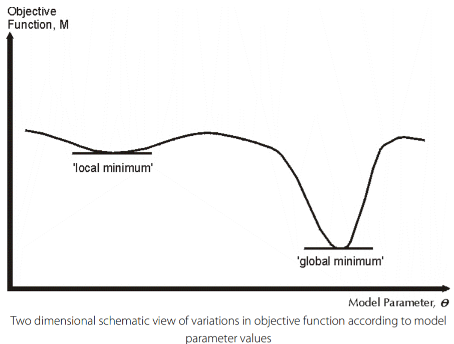
It is at this stage, in particular, that CUBE Analyst is operating in ”parameter space.” The principle is, simply, to adjust each parameter by an amount (the ”step length”) and by a search direction (up or down). The optimizer ensures that CUBE Analyst only makes adjustments which improve the situation (that is, to further minimize the objective function, M). Once a set of (improving) adjustments has been made, the CUBE Analyst optimizer performs another iteration of adjustments to determine whether more improvements are possible, and so on, until no further decrease in the (negative) value of the objective function is possible.

This approach places several requirements on the optimizer:

• Efficiency in determining optimum step lengths and directions
• Avoidance of ”local minima” and location of the ”global minimum” (this means being sure that no values of step length and direction could lead to a better result)
• Identification of the minimum point when in the neighborhood of one (this means achieving a stable convergence point)

There are several possible approaches to calculating optimum step lengths and directions. These may be considered to represent a spectrum characterized, at one end, by methods which use a simple strategy to define a step length and direction, but spend more time adjusting these elements through more iterations; at the other end, the methods spend more effort calculating the optimum step length and direction, but require fewer iterations.

The direction information is held by CUBE Analyst in the gradient search matrix file; this is also known as the Hessian matrix, as the gradient search matrix is an approximation for the Hessian. The degree of approximation depends on the method and certain aspects of the calculation, notably the proximity to convergence and the number of iterations since the gradient search was last re-computed (controlled in part by CUBE Analyst control parameter ITERH).

The significance of the Hessian matrix for CUBE Analyst is that it provides a mathematical description of the relationships between model parameters; indeed the Hessian itself approximates to the variance-covariance matrix. This can be exploited by the optimizer to update the direction information in an optimum manner.

Through the CUBE Analyst control parameter IHTYPE, the user can select alternative methods. These are listed below in order of increasing calculation effort given to the step length and direction:

1.Method of steepest descent

2.Newton’s method

3.Quasi-Newton method

4.Method of scoring.

The default procedure in CUBE Analyst uses a combination of methods (iii) and (iv). It starts by using the method of scoring to calculate an approximation to the Hessian, which requires considerable computational effort. Further improvements to the solution are obtained by the quasi-Newton method, which needs less computation. This method works well and requires very few iterations if the solution is in the region of the optimum value. Otherwise the gradient search matrix is recalculated using a method to determine the exact Hessian matrix, a new step length is adopted, and the process repeats itself. (If the exact Hessian cannot be computed, maybe because the results are still far from a converged solution, the method of scoring is automatically re-applied.)

As the solution approaches the optimum, the step length is reduced, allowing the optimum to be located more precisely. A very small step length indicates a close proximity to the optimum value and so the search is terminated when the step length is beneath the threshold defined by CUBE Analyst control parameter UTOL. This is a more practical method of determining when the calculation should finish than monitoring the gradients approaching zero.

Mathematical summary

This section presents a further explanation of CUBE Analyst’s calculations, as given in Introduction to the mathematics in CUBE Analyst.

Topics include:

• Maximum likelihood method: Background theory
• Application of maximum likelihood to CUBE Analyst
• CUBE Analyst objective function
• CUBE Analyst trip estimation model
• Estimating model parameters
• Optimization procedure
• Parameter errors
• Cell reliability

Maximum likelihood method: Background theory

Maximum likelihood is a standard method of estimating parameters of mathematical modeling equations, based on sets of relevant data observations. Given values of the model parameters, the pdf defines the probability associated with the observed data. When viewed as a function of the model parameters, the pdf is called a Likelihood function. The values of the parameters which maximize this function are called maximum likelihood estimates. They correspond to a model in which the probability of the observed data is maximized. The estimation process has two elements of establishing the likelihood function and of determining the optimum parameter values to maximize it.

Mathematically, the theory may be expressed as:

(4)

where:

X = random variable

x = observation

= parameter (or function of a parameter)

The likelihood function is then defined to be:

(5)

where:

that is, is a set of n observations

The optimization process is to find the value of that maximizes L

Application of maximum likelihood to CUBE Analyst

In accordance with the above theory, but with a slightly altered notation, the following are defined:

H = a data item (x =above)

h = an estimated item ( =above)

It is assumed that the appropriate pdf is

(6)

where is called the ”weighting factor.” It can be seen that is a Poisson random variable with mean . Thus can be considered a scaling parameter which defines the time units in the underlying Poisson process.

A likelihood function may thus be defined as:

(7)

Taking logarithms of equation (7) leads to:

(8)

It may be noted that = constant

Referring to equation (5), and considering all data items, H, a likelihood function may be defined as:

(9)

For computational ease, the task of maximizing L may be converted to the minimization of:

(10)

where

(11)

Equation (10) therefore represents the general form of the objective function which is minimized by CUBE Analyst.

CUBE Analyst objective function

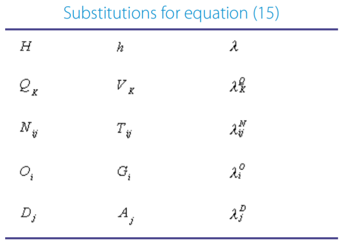
CUBE Analyst allows varied data items to be used in the estimation, that is, H and h may represent different data items, as shown in the following table:

Substituting these observed and estimated data items into Equation (10) gives an objective function shown below, with the source of the data indicated.

For reasons to do with function evaluation, the estimated tij is treated as a least squares minimization in the objective function. The objective function then becomes:

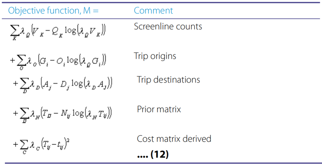
where indicates summation over cells which are zero in the prior matrix, but not the cost matrix.

CUBE Analyst trip estimation model

The objective function, equation (12) above, is used to calibrate the trip estimation model of the form:

(13)

where tij = Nij

or

Estimating model parameters

It follows, by differentiation of equation (11):

(14)

(15)

(Note: undefined for h=0)

The minimum value of the objective function, M, for a parameter , is found when

The remaining steps are to:

1.Calculate T_ij using equation (13) and current values of Model Parameters.

2.Use the table Observed data, H, and estimated equivalents, h to calculate h for each set of input and estimated data.

3.Calculate as we show below, for each set of estimated data.

leads to

(16)

where

(17)

and

(18)

Note: are constants

is undefined if V_k, T_ij, G_i or Aj=0.

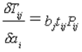
In equation (16) we need to substitute each set of model parameters for . We start by determining for each parameter reproducing Model Equation (13),

(13)

where t_ij= constant

or

let

Then differentiating (13) gives:

(for each ) a_i(19)

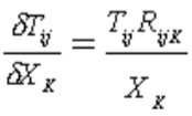(for each ) b_j(20)

(for )(21)

(22)

(23)

Finally, we substitute (19) to (23) into (16) for each value of , and use an optimization procedure to choose parameter values that give values T_ij of that minimize the objective function (9).

Optimization procedure

Given an initial guess CUBE Analyst computes the maximum likelihood estimates by generating a sequence of estimates from

where is a suitable step length, and denotes a search vector given by

For the method of scoring used by CUBE Analyst, is equal to the expected value of the Hessian matrix. It may be shown that this can be represented as

where E indicates the expected value, and , which denotes the gradient vector of the objective function, M, with respect to the model parameters, .

The(i,j) entry of the matrix is given by

(24)

From equation (16) we can write

(25)

This leads to

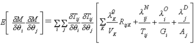(26)

The formulae for and are given in equations (19) to (23).

When is calculated by the quasi-Newton method (as previously described in Introduction to the mathematics in CUBE Analyst), the Hessian matrix updates the expected value, , using the BFGS update formula.

Parameter errors

The optimization produces an estimate z_p the variance of parameter image\help0189_wmf.gif, and an estimate of the parameter value itself,E_p.

Therefore,

Standard Error =(27)

and the range within ± one Standard Error is

Cell reliability

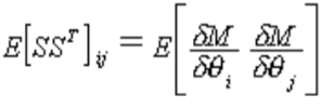
The ”sensitivity” of the estimate ofT_ij, S_ij, is defined to be

(28)

where L is the objective function, and represents a matrix of second differentials.

Extensions to the calculations

Hierarchic estimation is described in Chapter 7, “Hierarchic Estimation.”

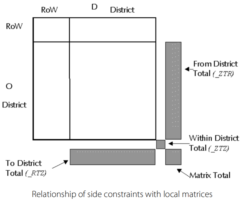
Hierarchic estimation calculates two forms of matrix, the district matrix and a set of local matrices. Apart from the aggregation of information which is implied by converting a zonal matrix to a district matrix, the estimation of a district matrix is entirely similar to a standard estimation. The estimation of the local matrices is, equally, similar, but it introduces a new set of data, derived from the district matrix, which are referred to as ”side constraints.”

To understand this ”side constraint” information, we show a local matrix in a schematic form in the following figure.

The set of side constraint variables, in terms of prior ”observed” (H) and estimated (h) data, and associated confidence levels, l, are:

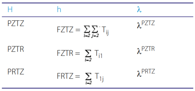
Note that the corresponding confidence levels,, and are all set by the user with CUBE Analyst’s ZCONF control parameter.

(The confidence levels for the trip ends applied to the district matrix are set according to the minimum values of the generation and attraction trip ends confidence levels found in the trip end file.)

These values of H and h are the substituted in the same manner which applies to other sets of data represented by H and h.